MNIST

Scripts

• mnist.q - script to read in MNIST data

• logit.q - single layer regression model to classify MNIST digits

• linear.q - 2-layer linear model

• conv.q - convolutional model

• swa.q - stochastic weight averaging of convolutional model

• simple.q - implementation of SimpNet with 13 convolutional layers

• gan.q - generative adversarial network to generate digits

• cgan.q - conditional generative adversarial network to generate digits by class

• lstm.q - alternate, recurrent form of model to classify digits

Data

The MNIST dataset is available here. The mnist.q - script assumes the downloaded binary files are uncompressed in a data/ directory that exists at the same level as the script. The directory should have the following files:

> ls -lh examples/mnist/data
total 53M
-rw-r--r-- 1 t t 7.5M May 17  2019 t10k-images-idx3-ubyte
-rw-r--r-- 1 t t 9.8K May 17  2019 t10k-labels-idx1-ubyte
-rw-r--r-- 1 t t  45M May 17  2019 train-images-idx3-ubyte
-rw-r--r-- 1 t t  59K May 17  2019 train-labels-idx1-ubyte

Loading

The mnist.q script loads a mnist() function that creates a dictionary of images and labels from the raw data files:

mnist(datadir) → k dictionary of mnist data

Parameters

datadir (symbol) – null to use default directory derived from the path of the calling script else a symbol prefixed with a colon, e.g. `:data.

Returns

A dictionary of smallints, with keys `x & `y for training images and labels, along with keys `X & `Y for test images and labels.

> q examples/mnist/mnist.q
KDB+ 4.0 2020.05.04 Copyright (C) 1993-2020 Kx Systems
l64/ 12(16)core 64037MB

q)d:mnist[]   /use default data directory

q)d~mnist`:examples/mnist/data
1b

q)d
x| 0 0 0 0 0 0 0 0 0 0 0 0 0 0 0 0 0 0 0 0 0 0 0 0 0 0 0 0 0 0 0 0 0 0 0 0 0 ..
y| 5 0 4 1 9 2 1 3 1 4 3 5 3 6 1 7 2 8 6 9 4 0 9 1 1 2 4 3 2 7 3 8 6 9 0 5 6 ..
X| 0 0 0 0 0 0 0 0 0 0 0 0 0 0 0 0 0 0 0 0 0 0 0 0 0 0 0 0 0 0 0 0 0 0 0 0 0 ..
Y| 7 2 1 0 4 1 4 9 5 9 0 6 9 0 1 5 9 7 3 4 9 6 6 5 4 0 7 4 0 1 3 1 3 4 7 2 7 ..

q)count each d
x| 47040000
y| 60000
X| 7840000
Y| 10000

q)2*sum count each d
109900000

q)-22!d
109900053

Dictionary keys `x, `y contain the 60,000 training images and labels (60,000 x 28 x 28 = 47,040,000), keys `X, `Y contain the 10,000 images and labels for testing the fitted model.

Quick display

The showdigit() will output a rough text display of a random digit from a set of images & labels:

q)showdigit . d`x`y
2h

          **********
         ***********
         *****   ****
         ***      ***
                  ***
                 ****
                *****
               *****
              ******
            ******
          ******
         *****
       *****
      *****
     *****
     ****
     ***
     *****************
      *****************
      *****************

Digit labels

The digits() function returns a font of digits 0-9 used to label output grids:

q)n:digits[]
q)-2@7_-7_6_'-6_' "* "0=n 9;

     *****
    *******
   **** ***
   ***  ****
   ***   ***
   ***   ***
   *********
    ********
     *******
        ***
    *******
    *******
     ****

Single layer

The logit.q script uses a single linear layer classify MNIST digits:

q)\l examples/mnist/mnist.q
q)d:mnist[`:examples/mnist/data]

q)count each d
x| 47040000
y| 60000
X| 7840000
Y| 10000

Scale pixels

The grayscale images are scaled to numbers between -1.0 and 1.0 and reshaped to 784 pixels each:

q)d:@[;`y`Y;"j"$]@[d;`x`X;{resize("e"$-1+x%127.5;-1 784)}]

q)count each d
x| 60000
y| 60000
X| 10000
Y| 10000

Model

A single linear layer is used for the model, along with the cross entropy loss function and the stochastic gradient descent optimizer:

q)q:module enlist(`linear;784;10)
q)elements q  /number of trainable parameters in model
7850

q)l:loss`ce
q)o:opt(`sgd;q;.04)
q)m:model(q;l;o)

Training

The batch size for training is set to 100 and the training data set is to be shuffled at each epoch:

q)train(m; `batchsize`shuffle; 100,1b)
q)train(m; d`x; d`y);

The model is run for 20 passes through the training data taken 100 images at a time, completing in a few seconds:

q)\ts:20 run m
1652 528

The output of the model in evaluation mode (no gradient calculation) is a matrix of weights (logits), 1 row per observation and and 1 column for each of the 10 possible digits:

q)y:evaluate(m; d`X)

q)count y
10000
q)count y 0
10

q)y
0.4986   -9.818 1.419   6.727     -2.822   0.384    -9.603  12.22   0.3794 3...
5.541    0.1578 12.02   5.854     -13.88   6.12     7.144   -18.24  5.024  -1..
-6.993   7.03   2.669   1.506     -2.313   0.1852   -0.3844 1.582   1.081  -1..
..

The predicted digit of the model is the column with the largest weight for each row:

q){x?max x}each evaluate(m; d`X)
7 2 1 0 4 1 4 9 6 9 0 6 9 0 1 5 9 7 3 4 9 6 6 5 4 0 7 4 0 1 3 1 3 6 7 2 7 1 2..

q)avg d.Y={x?max x}each evaluate(m; d`X)
0.9238

q)string[100*avg d.Y={x?max x}each evaluate(m; d`X)],"% test accuracy"
"92.38% test accuracy"

The single linear layer model usually achieves about 92% accuracy after 20 epochs, closer to 92.5% with 100 epochs. Run time on a 12-core i7 CPU is under 2 seconds.

Linear layers

The linear.q scripts creates a model of 2 linear layers with a relu activation function in between.

Model

The training images are treated as a list of 784 pixels and passed through each linear layer and the activation function.

• input: 100 x 784

• first linear layer: 100 x 784 x 784 x 800 -> 100 x 800

• relu: 100 x 800

• linear: 100 x 800 x 800 x 10 -> 100 x 10

q)q:module seq(`sequential; (`linear;784;800); `relu; (`linear;800;10))

q)-2 str q;
torch::nn::Sequential(
  (0): torch::nn::Linear(in_features=784, out_features=800, bias=true)
  (1): torch::nn::ReLU()
  (2): torch::nn::Linear(in_features=800, out_features=10, bias=true)
)

q)elements q
636010

Training

This model has 636,010 trainable parameters and usually converges to around 98.5% accuracy on the test dataset. The output is the same shape and type as in the single linear model in the logit.q script, but the depth and large increase in parameters makes for a better predictor:

> q examples/mnist/linear.q
KDB+ 4.0 2021.07.12 Copyright (C) 1993-2021 Kx Systems
l64/ 12(16)core 64033MB

  1.  loss: 0.269020  test: 0.1316  accuracy: 96.16%
  2.  loss: 0.127664  test: 0.1177  accuracy: 96.28%
  3.  loss: 0.094828  test: 0.1350  accuracy: 95.54%
  4.  loss: 0.081220  test: 0.0955  accuracy: 97.19%
  5.  loss: 0.068084  test: 0.1122  accuracy: 96.54%
 ..
 45.  loss: 0.000066  test: 0.0835  accuracy: 98.53%
 46.  loss: 0.000066  test: 0.0836  accuracy: 98.56%
 47.  loss: 0.000061  test: 0.0839  accuracy: 98.55%
 48.  loss: 0.000060  test: 0.0841  accuracy: 98.55%
 49.  loss: 0.000059  test: 0.0843  accuracy: 98.54%
 50.  loss: 0.000058  test: 0.0845  accuracy: 98.55%
9289 4195504

Run time on a NVIDIA GeForce GTX 1080 Ti GPU is around 10 seconds, closer to 30 seconds on a 12-core i7 CPU.

Convolutional model

The conv.q script builds a sequential model with two convolutional layers and a final set of two linear modules and a relu activation function in between.

Model

This model uses the training images as rectangles of 28 x 28 pixels, with the convolutions capturing more spatial information then the linear models in the logit.q and linear.q scripts.

q)q:(`sequential; (`conv2d; 1;20;5); `relu; `drop; (`maxpool2d;2))
q)q,:            ((`conv2d;20;50;5); `relu; `drop; (`maxpool2d;2); `flatten)
q)q,:            ((`linear;800;500); `relu; `drop; (`linear;500;10))

q)q:seq q  /enlist all but 1st

q)q
`sequential
,(`conv2d;1;20;5)
,`relu
,`drop
,(`maxpool2d;2)
,(`conv2d;20;50;5)
,`relu
,`drop
,(`maxpool2d;2)
,`flatten
,(`linear;800;500)
,`relu
,`drop
,(`linear;500;10)

The PyTorch’s representation of the model:

q)-2 str q;
torch::nn::Sequential(
  (0): torch::nn::Conv2d(1, 20, kernel_size=[5, 5], stride=[1, 1])
  (1): torch::nn::ReLU()
  (2): torch::nn::Dropout(p=0.5, inplace=false)
  (3): torch::nn::MaxPool2d(kernel_size=2, stride=2, padding=0, dilation=1)
  (4): torch::nn::Conv2d(20, 50, kernel_size=[5, 5], stride=[1, 1])
  (5): torch::nn::ReLU()
  (6): torch::nn::Dropout(p=0.5, inplace=false)
  (7): torch::nn::MaxPool2d(kernel_size=2, stride=2, padding=0, dilation=1)
  (8): torch::nn::Flatten(start_dim=1, end_dim=-1)
  (9): torch::nn::Linear(in_features=800, out_features=500, bias=true)
  (10): torch::nn::ReLU()
  (11): torch::nn::Dropout(p=0.5, inplace=false)
  (12): torch::nn::Linear(in_features=500, out_features=10, bias=true)
)

Training

Running the model for 50 epochs takes around 25 seconds on a single NVIDIA GeForce GTX 1080 Ti GPU with accuracy of around 99.6% Training on a 12-core i7 CPU takes around 6 minutes. A log of some training runs is available here.

KDB+ 4.0 2021.07.12 Copyright (C) 1993-2021 Kx Systems
l64/ 12(16)core 64033MB

 1.  lr: 0.0100  training loss: 0.827390  test accuracy: 96.84%
 2.  lr: 0.0100  training loss: 0.194377  test accuracy: 98.77%
 3.  lr: 0.0100  training loss: 0.154955  test accuracy: 98.88%
..
48.  lr: 0.0002  training loss: 0.087358  test accuracy: 99.61%
49.  lr: 0.0002  training loss: 0.087596  test accuracy: 99.60%
50.  lr: 0.0002  training loss: 0.087125  test accuracy: 99.64%

A dictionary of mismatches – keys for the digit and the corresponding mismatches predicted by the model – is output:

mismatches:
0| ,7
1| ,3
2| 1 7 7 7 7
3| ,5
4| ,9
5| 0 3 3 3 3 6
6| 0 0 1 4 5
7| 1 1 2 8
8| 3 9
9| 4 4 4 4 4 4 5 5 7 7

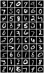
The grid of mismatches, examples/mnist/out/conv.png, is written to a .png file. The row labels are the model’s classification and the column labels are the actual digit. In the example below, most of the mismatches involve the digit 9, which the model mistakes for 4, 5 and 7.

Weight averaging

The swa.q script implements an example of stochastic weight averaging of the convolutional model used in the conv.q script.

The k-api implements weight averaging by taking a copy of the parameters at some point in the training and maintaining a running average after each epoch. At the end of training, the averaged parameters are written back to the model.

In this implementation, the convolutional model is trained for 50 epochs with weight averaging in effect for the final 20 epochs. While the averaging provides only a mild improvement over the regular training procedure (average accuracy of 99.592% vs 99.585%), the script is included to provide an example of the averaging technique using the k api.

The distribution of accuracy of 100 trials of the two training methods:

accuracy| regular averaging
--------| -----------------
99.45   | 1
99.51   |         1
99.53   | 6       3
99.54   | 5       5
99.55   | 9       9
99.56   | 9       7
99.57   | 14      4
99.58   | 3       10
99.59   | 14      11
99.6    | 12      11
99.61   | 9       14
99.62   | 4       12
99.63   | 5       4
99.64   | 6       4
99.65   |         3
99.66   | 1       1
99.68   | 1       1
99.71   | 1

A log of 100 trials using weight averaging is available here.

SimpNet

The paper Towards Principled Design of Deep Convolutional Networks: Introducing SimpNet proposes a simple network of convolutional layers followed by normalization layers. The model is implemented in the simple.q script, creating a deeper convolutional model than the implemention in conv.q.

Model

The model is build around a set of 13 convolutional layers, with additional batchnorm layers before the relu activation function and followed by a dropout layer and interspersed with max pooling layers after the 5th and 10th convlutions. The network finishes with a global max pooling layer and a linear layer to transform the model output into a matrix of one row per input image and 10 columns of weights for each digit.

The script builds a list of layer settings:

/ input output size pool
q:( 1    66    3    0;
   66    64    3    0;
   64    64    3    0;
   64    64    3    0;
   64    96    3    2;
   96    96    3    0;
   96    96    3    0;
   96    96    3    0;
   96    96    3    0;
   96   144    3    2;
  144   144    1    0;
  144   178    1    0;
  178   216    3    7)

And defines a helper function to translate the settings into a set of layers:

f:{[i;o;s;p]
 c:(`conv2d;i;o;s;1;`same);      /convolution layer w'padding=same
 b:(`batchnorm2d;o;1e-05;.05);   /batchnorm w'momentum of .95
 f:`relu; d:(`drop;.2); m:(`maxpool2d;p);
 / final global max pool needs reshape & linear layer
 if[p=7; r:(`reshape;-1,o); l:(`linear;o;10)];
 $[p=0; (c;b;f;d); p=2; (c;b;f;m;d); (c;b;f;m;r;d;l)]}

q)f . q 0
(`conv2d;1;66;3;1;`same)
(`batchnorm2d;66;1e-05;0.05)
`relu
(`drop;0.2)

q)f . last q
(`conv2d;178;216;3;1;`same)
(`batchnorm2d;216;1e-05;0.05)
`relu
(`maxpool2d;7)
(`reshape;-1 216)
(`drop;0.2)
(`linear;216;10)

The layers are all defined as child modules of one sequential container:

q)`sequential,enlist each raze f ./:q
`sequential
,(`conv2d;1;66;3;1;`same)
,(`batchnorm2d;66;1e-05;0.05)
,`relu
,(`drop;0.2)
,(`conv2d;66;64;3;1;`same)
,(`batchnorm2d;64;1e-05;0.05)
,`relu
,(`drop;0.2)
..
`conv2d 144 178 1 1 `same
`batchnorm2d 178 1e-05 0.05
relu
`drop 0.2
`conv2d 178 216 3 1 `same
`batchnorm2d 216 1e-05 0.05
relu
`maxpool2d 7
`reshape -1 216
`drop 0.2
`linear 216 10

The PyTorch representation of the model is here.

Training

Comparing the SimpNet model to the one in the conv.q script, there is an increase in trainable parameters from around 400,000 to 1 million. But it is the depth of the SimpNet model that has more of an impact on training time: the simpler convolutional model uses 13 layers whereas the SimpNet model uses 57 layers. The increased depth of the model increases training time to 17 seconds per epoch, about 14 minutes for 50 epochs for an accuracy increase from around 99.6% to 99.7% (a log of some training runs using a NVIDIA GeForce GTX 1080 Ti GPU is available here).

> q examples/mnist/simple.q
KDB+ 4.0 2021.07.12 Copyright (C) 1993-2021 Kx Systems
l64/ 12(16)core 64033MB

epochs: 50, batch size: 100, iterations per epoch: 600
  1.  lr: 0.0100  training loss: 0.503514  test accuracy: 94.19%
  2.  lr: 0.0100  training loss: 0.166132  test accuracy: 95.26%
  3.  lr: 0.0100  training loss: 0.148934  test accuracy: 97.09%
 ..
 47.  lr: 0.0002  training loss: 0.080834  test accuracy: 99.69%
 48.  lr: 0.0001  training loss: 0.080072  test accuracy: 99.74%
 49.  lr: 0.0000  training loss: 0.079776  test accuracy: 99.72%
 50.  lr: 0.0000  training loss: 0.079329  test accuracy: 99.73%

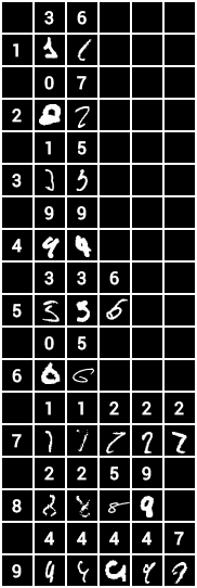
mismatches:
1| 3 6
2| 0 7
3| 1 5
4| 9 9
5| 3 3 6
6| 0 5
7| 1 1 2 2 2
8| 2 2 5 9
9| 4 4 4 4 7

grid of mismatches: examples/mnist/out/simple.png

Weight averaging

A weight averaging version of the model trains for 75 epochs, with the average of the weights for the final 25 epochs used as the model parameters. A training run of the weighted average version is here, along with a grid of mismatches.

GAN

The gan.q script builds a Generative Adverserial Network (GAN). It consists of a discriminator model and a generator model to create new MNIST digits using random inputs: the generator model is trained to convince the discriminator model that the digits are part of the handwritten dataset.

Model

Define convolution sizes and a helper function to build both generator and discriminator models:

q)n:100 256 128 64
q)gan:{to(x:module seq `sequential,x;y); model(x; loss`bce; opt(`adam;x;.0002;.5))}

Define the generator layers:

q)a:`pad`bias!(1;0b)
q)g :((`convtranspose2d;n 0;n 1;4;1_a); (`batchnorm2d;n 1); `relu)  / 256 x  4 x  4
q)g,:((`convtranspose2d;n 1;n 2;3;2;a); (`batchnorm2d;n 2); `relu)  / 128 x  7 x  7
q)g,:((`convtranspose2d;n 2;n 3;4;2;a); (`batchnorm2d;n 3); `relu)  /  64 x 14 x 14
q)g,:((`convtranspose2d;n 3;  1;4;2;a); `tanh)                      /   1 x 28 x 28

q)g:gan[g]`cpu

The generator is designed to take random noise and generate 28 x 28 images that resemble the MNIST handwritten digits:

q)z:tensor(`randn;60 100 1 1)

q)x:forward(g;z)

q)size x
60 1 28 28

The adversarial design of a GAN requires an accompanying discriminator:

q)a:`bias,0b
q)d :((`conv2d;  1;n 3;4;2;1;a); (`leakyrelu; 0.2))                      /  64 x 14 x 14
q)d,:((`conv2d;n 3;n 2;4;2;1;a); (`batchnorm2d;n 2); (`leakyrelu; 0.2))  / 128 x  7 x  7
q)d,:((`conv2d;n 2;n 1;4;2;1;a); (`batchnorm2d;n 1); (`leakyrelu; 0.2))  / 256 x  3 x  3
q)d,:((`conv2d;n 1;  1;3;1;0;a); `sigmoid; (`flatten;0))                 /   1 x  1 x  1

q)d:gan[d]`cpu

The discriminator is designed to take handwritten digits or generated digits and return a number close to 1 for handwritten digits and close to 0 if generated.

q)z:tensor(`randn;60 100 1 1)
q)x:forward(g;z)

q)y:forward(d;x)

q)size y
,60
q)tensor y
0.3427 0.5647 0.3511 0.4858 0.2941 0.3766 0.3467 0.3052 0.4612 0.4087 0.3725 ..

The PyTorch representation of the generator and discriminator is here.

Training

After the generator and discriminator models are defined, the training proceeds in three steps:

• train discriminator with handwritten images as inputs and targets close to 1.0 (fit1)

• train discriminator again with generated images as inputs and targets of 0.0 (fit2)

• train the generator via the gradients from the discriminator using generated images and targets of 1.0 (fit3)

These steps are defined in fit1, fit2 and fit3, called in turn by the function fit:

fit1:{[d;x;y] nograd d; uniform(y;.8;1); backward(d;x;y)}
fit2:{[d;x;y] x:detach x; l:backward(d;x;y); free x; step d; l}
fit3:{[d;g;x;y] nograd g; l:backward(d;x;y); free x; step g; l}

fit:{[d;g;t;x;z;w;i]
/d:discriminator, g:generator, t:targets, x:images, z:noise, w:batch size, i:index
 batch(x;w;i);             /take i'th subset of MNIST images
 l0:fit1[d;x;t 0];         /train discriminator w'real images
 normal z; x:forward(g;z); /generate images from noise
 l1:fit2[d;x;t 1];         /train d w'generated images
 l2:fit3[d;g;x;t 2];       /train generator w'discriminator accepting generated images
 (l0+l1),l2}               /return discriminator & generator loss

The training output from running for 20 passes through the set of 60,000 handwritten & generated images:

> q examples/mnist/gan.q
KDB+ 4.0 2021.07.12 Copyright (C) 1993-2021 Kx Systems
l64/ 12(16)core 64033MB

Epochs: 20, batch size: 60, iterations per epoch: 1000
Epoch: 1    10:11:55    Median loss for discriminator: 0.763 generator: 2.026
Epoch: 2    10:12:02    Median loss for discriminator: 0.712 generator: 1.473
Epoch: 3    10:12:09    Median loss for discriminator: 0.682 generator: 1.879
Epoch: 4    10:12:16    Median loss for discriminator: 0.667 generator: 1.624
Epoch: 5    10:12:23    Median loss for discriminator: 0.653 generator: 2.126
Epoch: 6    10:12:30    Median loss for discriminator: 0.635 generator: 2.829
Epoch: 7    10:12:37    Median loss for discriminator: 0.607 generator: 2.334
Epoch: 8    10:12:44    Median loss for discriminator: 0.610 generator: 2.524
Epoch: 9    10:12:51    Median loss for discriminator: 0.589 generator: 2.558
Epoch: 10   10:12:58    Median loss for discriminator: 0.606 generator: 3.371
Epoch: 11   10:13:05    Median loss for discriminator: 0.577 generator: 2.708
Epoch: 12   10:13:12    Median loss for discriminator: 0.564 generator: 2.534
Epoch: 13   10:13:19    Median loss for discriminator: 0.556 generator: 3.406
Epoch: 14   10:13:26    Median loss for discriminator: 0.551 generator: 2.644
Epoch: 15   10:13:33    Median loss for discriminator: 0.544 generator: 3.241
Epoch: 16   10:13:40    Median loss for discriminator: 0.531 generator: 2.638
Epoch: 17   10:13:47    Median loss for discriminator: 0.535 generator: 3.336
Epoch: 18   10:13:54    Median loss for discriminator: 0.525 generator: 3.293
Epoch: 19   10:14:01    Median loss for discriminator: 0.528 generator: 3.681
Epoch: 20   10:14:08    Median loss for discriminator: 0.510 generator: 3.458

Generated digits in dir examples/mnist/out/, gan01.png - gan20.png, gan.gif

The script produces a grid of generated images after each epoch and creates a GIF file that shows each epoch in succession (requires convert utility). Each grid depicts the digits generated by the same set of random variables used at the end of each epoch:

Epoch 1	Epoch 5	Epoch 10	Epoch 20	1 to 20

Conditional GAN

The cgan.q script builds a generator and discriminator model similar to the models in gan.q, but conditioning the images with their class so that images can be generated and evaluated with their accompanying target digit included in the input.

Model

The generator and discriminator use a k api module seqjoin to define the processing of the class 0-9 and how this part of the input is combined with the random numbers used in the generator and the images used as input to the discriminator.

For the generator module the random noise is joined with the target digit via a learned embedding and a reshape so that the two tensors can be catenated together:

e:10

g:((0; `sequential);
   (1; `seqjoin);
   (2; `sequential);          / 1st fork: random vars
   (2; `sequential);          / 2nd fork: digit
   (3; (`embed;10;e));
   (3; (`reshape;-1,e,1,1));
   (2; (`cat;1));             / join inputs
..

For the discriminator, a wider embedding is used, along with a linear layer, then a reshape to create tensors of batchsize x channel x height x width which are catenated together:

e:50

d:((0; `sequential);
   (1; `seqjoin);
   (2; `sequential);     / 1st fork: images passed through empty sequential
   (2; `sequential);     / 2nd fork: digit -> embedding -> liner -> 28 x 28
   (3; (`embed;10;e));
   (3; (`linear;e;28*28));
   (3; (`reshape;-1 1 28 28));
   (2; (`cat;1));
   ..

Once the inputs of noise & digit for the generator, and image & digit for the discriminator are catenated together, the remainder of the models are a series of convolutions or transposed convolutions, followed by normalization layers and relu or leakyrelu activations.

The PyTorch representation of the generator and discriminator modules is available here.

Training

After the generator and discriminator models are defined, the training proceeds in the same three steps used by the gan.q script, but with the addition of the digits 0-9 accompanying the random noise of the generator or the images of the discriminator:

• train discriminator with handwritten images & labels as joint inputs and targets close to 1.0 (fit1)

• train discriminator again with generated images & labels as inputs and targets of 0.0 (fit2)

• train the generator via the gradients from the discriminator using generated images & lables and targets of 1.0 (fit3)

These steps are defined in fit1, fit2 and fit3, called in turn by the function fit:

fit1:{[d;t;v] nograd d; uniform(t;0.8;1.0); backward(d;v;t)}
fit2:{[d;t;x;y] x:detach x; l:backward(d;(x;y);t); free x; step d; l}
fit3:{[d;g;t;x;y] nograd g; l:backward(d;(x;y);t); free(x;y); step g; l}

fit:{[d;g;t;v;z;w;i]
 batch(v;w;i);                              /i'th subset of MNIST images & labels
 l1:fit1[d;t 0;v];                          /train on real images
 normal z; y:tensor(`randint;10;w;c,`long); /random inputs & labels
 x:forward(g;z;y);                          /generate images
 l2:fit2[d;t 1;x;y];                        /train discriminator w'generated images & labels
 l3:fit3[d;g;t 2;x;y];                      /train generator: get discriminator to recognize as real
 (l1+l2),l3}                                /discriminator & generator loss

> q examples/mnist/cgan.q
KDB+ 4.0 2021.07.12 Copyright (C) 1993-2021 Kx Systems
l64/ 12(16)core 64033MB

Epochs: 20, batch size: 60, iterations per epoch: 1000
Epoch: 1    09:54:00    Median loss for discriminator: 0.947 generator: 1.494
Epoch: 2    09:54:08    Median loss for discriminator: 1.136 generator: 1.325
Epoch: 3    09:54:15    Median loss for discriminator: 1.146 generator: 0.880
Epoch: 4    09:54:23    Median loss for discriminator: 1.144 generator: 1.235
Epoch: 5    09:54:30    Median loss for discriminator: 1.139 generator: 1.388
Epoch: 6    09:54:38    Median loss for discriminator: 1.124 generator: 1.453
Epoch: 7    09:54:45    Median loss for discriminator: 1.096 generator: 1.298
Epoch: 8    09:54:53    Median loss for discriminator: 1.066 generator: 1.707
Epoch: 9    09:55:00    Median loss for discriminator: 1.043 generator: 1.814
Epoch: 10   09:55:08    Median loss for discriminator: 1.013 generator: 1.496
Epoch: 11   09:55:16    Median loss for discriminator: 0.971 generator: 1.598
Epoch: 12   09:55:23    Median loss for discriminator: 0.932 generator: 2.290
Epoch: 13   09:55:31    Median loss for discriminator: 0.899 generator: 2.212
Epoch: 14   09:55:38    Median loss for discriminator: 0.876 generator: 1.867
Epoch: 15   09:55:46    Median loss for discriminator: 0.843 generator: 1.691
Epoch: 16   09:55:54    Median loss for discriminator: 0.831 generator: 2.061
Epoch: 17   09:56:01    Median loss for discriminator: 0.811 generator: 1.649
Epoch: 18   09:56:09    Median loss for discriminator: 0.787 generator: 2.345
Epoch: 19   09:56:17    Median loss for discriminator: 0.770 generator: 2.343
Epoch: 20   09:56:24    Median loss for discriminator: 0.759 generator: 2.244

Generated digits in dir examples/mnist/out/, cgan01.png - cgan20.png, cgan.gif

Run time is about 2.5 minutes on a NVIDIA GeForce GTX 1080 Ti GPU and closer to 40 minutes on 12-core i7 CPU.

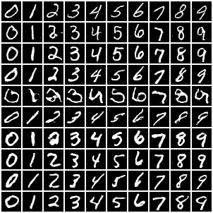
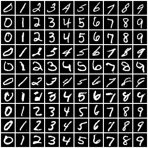
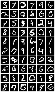
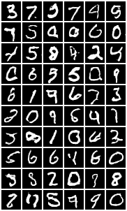
The script produces a grid of generated images after each epoch and creates a GIF file that shows each epoch in succession (requires convert utility). The rows of each grid are generated by the same set of random variables conditioned by the different digits 0-9; each column represents different images of the same digit generated by different randome variables:

Epoch 1	Epoch 10	Epoch 20	1 to 20

Recurrent Model

The lstm.q script uses a recurrent neural network to classify the digits. Each row of the 28 x 28 pixel images can be used as a sequence to demonstrate the recurrent architecture with a familiar dataset.

Model

The k-api container module, recur is used to first call the PyTorch lstm module and then the output sequence of the select of the final column and the linear transformation into a matrix of 10 columns of weights for each image.

q:module`recur
module(q; 1; (`lstm;     `lstm; 28; 128; 2; 1b; 1b))
module(q; 1;  `sequential);
module(q; 2; (`select;   `last; 1; -1))
module(q; 2; (`linear;   `decode; 128; 10))

q)-2 str q;
knn::Recur(
  (lstm): (input_size=28, hidden_size=128, num_layers=2, bias=true,..
  (out): torch::nn::Sequential(
    (last): knn::Select(dim=1,ind=-1)
    (decode): torch::nn::Linear(in_features=128, out_features=10, bias=true)
  )
)

Using a 60 x 28 x 28 tensor of random numbers as a placeholder for 60 MNIST images of digits, the first forward calculation uses the lstm module to get the output and hidden state:

q)x:tensor(`randn;60 28 28)
q)y:forward(q;`lstm;x)

q)size y
60 28 128
2  60 128
2  60 128

The result, y, is a vector of 3 tensors, the output of the lstm and the hidden and cell state of the sequence. The final column of the output is selected and passed through a linear layer to get the weights for each digit:

q)z:forward(q;`out;(y;0))

q)size z
60 10

Each subsequent call to the lstm module can include the hidden & cell state of the previous sequence:

q)vector(y; 0; tensor(`randn;60 28 28))

q)use[y]forward(q;`lstm;y)

q)size y
60 28 128
2  60 128
2  60 128

Training

The script uses a cycling learning rate, using .001, .0005, .0002, .0001 repeatedly for 40 iterations through the data. A recurrent model is not as accurate as the convolutional model, with an accuracy of 99.20 - 99.30%, running through 40 epochs in around 2 minutes on a NVIDIA GeForce GTX 1080 Ti GPU and 13 minutes on 12-core i7 CPU.

KDB+ 4.0 2021.07.12 Copyright (C) 1993-2021 Kx Systems
l64/ 12(16)core 64033MB

  1.  lr: 0.0010  training loss: 0.392026  test accuracy: 95.79%
  2.  lr: 0.0005  training loss: 0.087590  test accuracy: 97.74%
  3.  lr: 0.0002  training loss: 0.053733  test accuracy: 98.29%
  4.  lr: 0.0001  training loss: 0.038863  test accuracy: 98.49%
  5.  lr: 0.0010  training loss: 0.090845  test accuracy: 97.88%
 ..
 36.  lr: 0.0001  training loss: 0.001683  test accuracy: 99.25%
 37.  lr: 0.0010  training loss: 0.023589  test accuracy: 99.01%
 38.  lr: 0.0005  training loss: 0.007428  test accuracy: 99.23%
 39.  lr: 0.0002  training loss: 0.002182  test accuracy: 99.27%
 40.  lr: 0.0001  training loss: 0.001296  test accuracy: 99.32%
108020 4195680

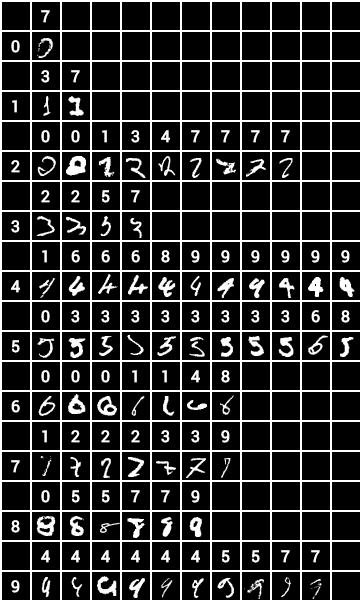
mismatches:
0| ,7
1| 3 7
2| 0 0 1 3 4 7 7 7 7
3| 2 2 5 7
4| 1 6 6 6 8 9 9 9 9 9 9
5| 0 3 3 3 3 3 3 3 3 6 8
6| 0 0 0 1 1 4 8
7| 1 2 2 2 3 3 9
8| 0 5 5 7 7 9
9| 4 4 4 4 4 4 5 5 7 7

grid of mismatches: examples/mnist/out/lstm.png

The grid of mismatches, examples/mnist/out/lstm.png, is written to a .png file. The row labels are the model’s classification and the column labels are the actual digit.